Exploration of Kepler dynamics with a Neural network
(by Sean Cowan)
This notebook investigates the 2D Kepler ODE system (in polar coordinates). In particular, we look at adding a perturbative acceleration in the form of a neural network. The equations are
which describes, in non dimensional units, the Keplerian motion of a mass point object around some primary body with a perturbation.
Importing stuff
[1]:
import time
import copy
import numpy as np
import matplotlib.pyplot as plt
import seaborn as sns
import matplotlib.colors as col

from scipy.integrate import solve_ivp

from pyaudi import gdual_double as gdual, taylor_model, int_d, sin, cos
from plotting_functions import plot_n_to_2_solution_enclosure, sample_on_square_boundary
Define Neural Network stuff
We define weights and biases congruent with a list (e.g. [4, 10, 2]) defining the size of the network, which is then used in ml_predict to produce an output given an input. We also define the ReLu activation function for more realism (but of course it works without).
[2]:
seed = 41+6  # Set your desired seed
rng = np.random.Generator(np.random.MT19937(seed))

def initialize_weights(n_units):
    weights = []

    for layer in range(1, len(n_units)):
        W_layer = np.empty((n_units[layer-1], n_units[layer]), dtype=object)
        for i in range(n_units[layer-1]):
            for j in range(n_units[layer]):
                symname = f'w_{{({layer},{j},{i})}}'
                exp_point = rng.uniform(low=-1, high=1)
                w_tm = exp_point
                W_layer[i, j] = w_tm
        weights.append(W_layer)

    return weights

def initialize_biases(n_units):
    biases = []

    for layer in range(1, len(n_units)):
        b_layer = np.empty((1, n_units[layer]), dtype=object)
        for j in range(n_units[layer]):
            symname = f'b_{{({layer},{j})}}'
            exp_point = 1
            b_tm = exp_point
            b_layer[0, j] = b_tm
        biases.append(b_layer)

    return biases

def ReLu(x):
    if isinstance(x, np.ndarray) and isinstance(x[0, 0], taylor_model):
        old_shape = x.shape
        x = x.reshape(-1, 1)
        for it, t in enumerate(x[:, 0]):
            if t.tpol.constant_cf > 0:
                pass
            else:
                x[it, 0] = 0
        return x.reshape(old_shape)
    elif isinstance(x, np.ndarray) and isinstance(x[0, 0], float):
        return np.where(x > 0, x, 0)
    elif isinstance(x, taylor_model):
        return x if x.tpol.constant_cf > 0 else 0
    elif isinstance(x, float):
        if x > 0:
            return x
        else:
            return 0
    else:
        raise RuntimeError(f"The input {x} of type {type(x)} is not valid.")

def ml_predict(x_in, W, b):
    layer_output = x_in
    for W_layer, b_layer in zip(W, b):
        layer_output = ReLu(layer_output @ W_layer + b_layer)
        # layer_output = layer_output @ W_layer
    return layer_output
Integration function
[3]:
def rk4_t(f, t0, y0, th):
    t = th
    timesteps = [(th[i + 1] - th[i]).item() for i in range(len(th) - 1)]
    y = np.array([[type(y0[0])] * np.size(y0)] * (len(t)))
    y[0] = y0
    for n in range(len(t) - 1):
        h = timesteps[n]
        xi1 = y[n]
        f1 = f(t[n], xi1)
        xi2 = y[n] + (h / 2.0) * f1
        f2 = f(t[n], xi2)
        xi3 = y[n] + (h / 2.0) * f2
        f3 = f(t[n], xi3)
        xi4 = y[n] + h * f3
        f4 = f(t[n], xi4)
        y[n + 1] = y[n] + (h / 6.0) * (f1 + 2 * f2 + 2 * f3 + f4)
    return y

minimum_network = [4, 1, 2]
default_weights = initialize_weights(minimum_network)
default_biases = initialize_biases(minimum_network)

def rk4_t_nn(f, t0, y0, th, f_args=(default_weights, default_biases, 1e-5)):
    t = th
    timesteps = [(th[i + 1] - th[i]).item() for i in range(len(th) - 1)]
    y = np.array([[type(y0[0])] * np.size(y0)] * (len(t)))
    y[0] = y0
    for n in range(len(t) - 1):
        h = timesteps[n]
        xi1 = y[n]
        f1 = f(t[n], xi1, *f_args)
        xi2 = y[n] + (h / 2.0) * f1
        f2 = f(t[n], xi2, *f_args)
        xi3 = y[n] + (h / 2.0) * f2
        f3 = f(t[n], xi3, *f_args)
        xi4 = y[n] + h * f3
        f4 = f(t[n], xi4, *f_args)
        y[n + 1] = y[n] + (h / 6.0) * (f1 + 2 * f2 + 2 * f3 + f4)
    return y
Define problem
[4]:
def eom_kep_polar(t, y):
    return np.array(
        [y[1], -1 / y[0] / y[0] + y[0] * y[3] * y[3], y[3], -2 * y[3] * y[1] / y[0]]
    )

def eom_kep_polar_thrust(t, y, weights=default_weights, biases=default_biases, max_thrust=1e-5):
    u = max_thrust * ml_predict(y.reshape(1, -1), weights, biases).reshape(-1)
    return np.array(
        [y[1], -1 / y[0] / y[0] + y[0] * y[3] * y[3] + u[0], y[3], -2 * y[3] * y[1] / y[0] + u[1]]
    )

# Order of Taylor series
order = 5
# Tolerance
tol=1e-10
# Neural network size
n_units = [4, 32, 32, 32, 2]
# Maximum thrust acceleration
max_thrust = 1e-3
# Number of orbits to propagate with random acceleration
n_samples = 4
# Size of valid domain for Taylor model
domain_size = 0.001

# The initial conditions
ic = [1.0, 0.1, 0.0, 1.0]
initial_time = 0.0
final_time = 5
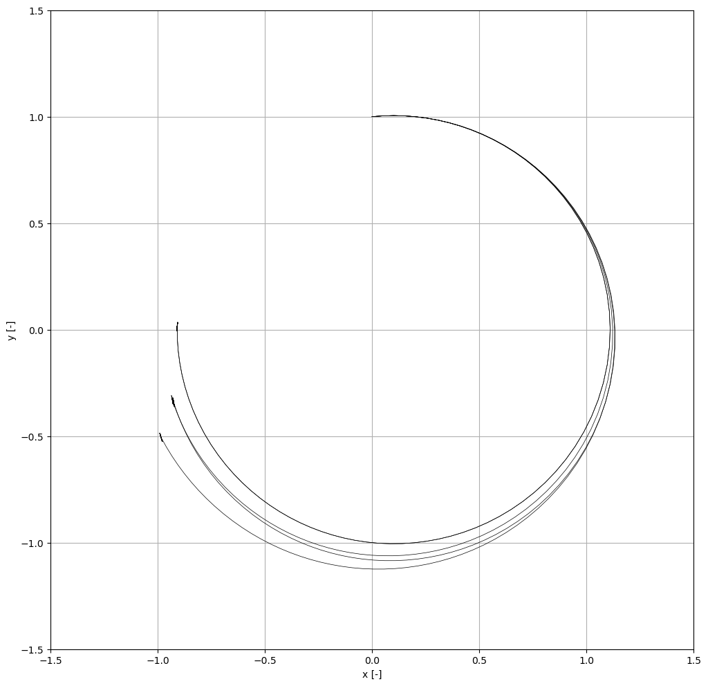
Numerical propagation
[5]:
y_num_viz = solve_ivp(
    eom_kep_polar, (initial_time, final_time), ic, method="RK45", rtol=1e-13, atol=1e-13
)
Taylor model propagation
Next, we propagate the Taylor models for a number of samples with randomised neural network weights and biases.
[6]:
fig, ax = plt.subplots(1, 1, figsize=(12, 12))

y_num = solve_ivp(
    eom_kep_polar, (initial_time, final_time), ic, method="RK45", rtol=tol, atol=tol
)

weights_list = []
biases_list = []
tm_list = []
for it in range(n_samples+1):

    weights = initialize_weights(n_units)
    weights_list.append(weights)
    biases = initialize_biases(n_units)
    biases_list.append(biases)

    symbols = ["r", "vr", "t", "vt"]
    ic_g = [
        gdual(ic[0], symbols[0], order),
        gdual(ic[1], symbols[1], order),
        gdual(ic[2], symbols[2], order),
        gdual(ic[3], symbols[3], order),
    ]
    ic_tm = [
        taylor_model(
            ic_g[i],
            int_d(0.0, 0.0),
            {symbols[i]: ic[i]},
            {symbols[i]: int_d(ic[i] - domain_size / 2, ic[i] + domain_size / 2)},
        )
        for i in range(4)
    ]

    # Only propagate r and theta as Taylor models.
    ic_tm[1] = ic[1]
    ic_tm[3] = ic[3]

    # We call the numerical integrator, this time it will compute on Taylor models
    if it == 0:
        y_tm = rk4_t(eom_kep_polar, initial_time, ic_tm, y_num.t)
    else:
        y_tm = rk4_t_nn(eom_kep_polar_thrust, initial_time, ic_tm, y_num.t, (weights, biases,
                                                                          max_thrust))
    tm_list.append(y_tm)
    nom_x1 = []
    nom_x2 = []
    for it2, y_step in enumerate(y_tm):

        r_step, vr_step, t_step, vt_step = y_step
        x_step = r_step * sin(t_step)
        y_step = r_step * cos(t_step)
        x1_tm = x_step
        x2_tm = y_step

        nom_x1.append(x1_tm.tpol.constant_cf)
        nom_x2.append(x2_tm.tpol.constant_cf)

        if it2 == len(y_tm) - 1 or it2 == 0:
            ax = plot_n_to_2_solution_enclosure(x1_tm, x2_tm, ax=ax, color="k", resolution=300)

    ax.plot(nom_x1, nom_x2, c='k', linewidth=0.5)

ax.set_xlim([-1.5, 1.5])
ax.set_ylim([-1.5, 1.5])
ax.set_xlabel("x [-]")
ax.set_ylabel("y [-]")
ax.grid()
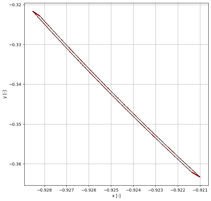
Finally, we take one of these samples and verify its behaviour with Monte Carlo shooting.
NOTE: Since we are using a numerical integrator, of which the integration error is not bounded, At very high precisions the Monte Carlo samples may fall outside the remainder bound in certain cases.
[7]:
sample = 3

fig, ax = plt.subplots(1, 1, figsize=(8, 8))

y_num = solve_ivp(
    eom_kep_polar, (initial_time, final_time), ic, method="RK45", rtol=tol, atol=tol
)

y_tm = tm_list[sample]
for it2, y_step in enumerate(y_tm):

    r_step, vr_step, t_step, vt_step = y_step
    x_step = r_step * sin(t_step)
    y_step = r_step * cos(t_step)
    x1_tm = x_step
    x2_tm = y_step

    if it2 == len(y_tm) - 1:
        ax = plot_n_to_2_solution_enclosure(x1_tm, x2_tm, ax=ax, color="k", resolution=300)

# Monte Carlo
n_samples_mc = int(1e3)

seed2 = 2
rng2 = np.random.Generator(np.random.MT19937(seed2))
ic_mc = copy.deepcopy(ic)

ic_r_th = sample_on_square_boundary([ic_mc[0], ic_mc[2]], domain_size, n_samples_mc=n_samples_mc, rng=rng2)

xfs = ic_r_th[0, :] * np.sin(ic_r_th[1, :])
yfs = ic_r_th[0, :] * np.cos(ic_r_th[1, :])

weights = weights_list[sample]
biases = biases_list[sample]
for j in range(n_samples_mc):
    current_ic = [ic_r_th[0, j], ic[1], ic_r_th[1, j], ic[3]]

    if sample == 0:
        y = rk4_t(eom_kep_polar, initial_time, current_ic, y_num.t).astype(float)
    else:
        y = rk4_t_nn(eom_kep_polar_thrust, initial_time, current_ic, y_num.t, (weights, biases,
                                                                           max_thrust)).astype(float)

    r = y[-1, 0]
    th = y[-1, 2]
    xfs = r * np.sin(th)
    yfs = r * np.cos(th)
    ax.scatter(xfs, yfs, c="r", s=0.5)

ax.set_xlabel("x [-]")
ax.set_ylabel("y [-]")
ax.grid()