Map (series) inversion

(by Dario Izzo)

In this notebook we show how to use the map inversion algorithm to locally invert systems of non linear equations.

Importing stuff

from pyaudi import gdual_double as gdual
from pyaudi import sin, cos
from pyaudi import invert_map

The Double Pendulum end-point

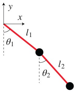
Let us consider, in 2D, the end point position of a double pendulum.

$$\begin{split}x = l_1 sin(\theta_1) + l_2 sin(\theta_2) \\ y = -l_1 cos(\theta_1) - l_2 cos(\theta_2)\end{split}$$

We will develop a model for the inversion of this system of equations, so that $\theta_1$ and $\theta_2$ can be expressed as a function of $x$ and $y$

# We show an image for clarity
from IPython.display import Image
from IPython.core.display import HTML
Image(url= "http://www.physicsandbox.com/assets/images/pendulum.jpg")

Define our variables

# Lengths for the pendulum arms
L1 = 1.
L2 = 1.3
# Nominal values for thetas
th1n = 0.3
th2n = -0.2
# Gduals (high order)
th1 = gdual(th1n, "\\theta_1", 11)
th2 = gdual(th2n, "\\theta_2", 11)
# Equations
x = L1*sin(th1)+L2*sin(th2)
y = -L1*cos(th1)-L2*cos(th2)

# Lets visualize the Taylor polinomial expansion for x
x

$$1.27409{d\theta_2}+2.63265e-06{d\theta_1}^{9}-0.000410445{d\theta_1}^{6}+3.51104e-06{d\theta_2}^{9}-0.159223{d\theta_1}^{3}+0.0372501+0.000358709{d\theta_2}^{6}-0.000252795{d\theta_2}^{7}-0.212348{d\theta_2}^{3}-2.39332e-08{d\theta_1}^{11}+7.32937e-06{d\theta_1}^{8}+0.00796114{d\theta_1}^{5}-0.0107613{d\theta_2}^{4}-0.14776{d\theta_1}^{2}+0.0106174{d\theta_2}^{5}-8.14374e-08{d\theta_1}^{10}-6.40551e-06{d\theta_2}^{8}-0.000189551{d\theta_1}^{7}+0.0123133{d\theta_1}^{4}+0.955336{d\theta_1}+\ldots+\mathcal{O}\left(12\right)$$

# Lets visualize the Taylor polinomial expansion for y
y

$$-0.25827{d\theta_2}+8.14374e-07{d\theta_1}^{9}+0.00132686{d\theta_1}^{6}-7.11723e-07{d\theta_2}^{9}-0.0492534{d\theta_1}^{3}-2.22942+0.00176956{d\theta_2}^{6}+5.12441e-05{d\theta_2}^{7}+0.043045{d\theta_2}^{3}-7.4034e-09{d\theta_1}^{11}-2.36939e-05{d\theta_1}^{8}+0.00246267{d\theta_1}^{5}-0.0530869{d\theta_2}^{4}+0.477668{d\theta_1}^{2}-0.00215225{d\theta_2}^{5}+2.63265e-07{d\theta_1}^{10}-3.15994e-05{d\theta_2}^{8}-5.8635e-05{d\theta_1}^{7}-0.0398057{d\theta_1}^{4}+0.29552{d\theta_1}+\ldots+\mathcal{O}\left(12\right)$$

Compute the inverse map

# And let us invert the relationship
res = invert_map([x,y])
th1_map = res[0]
th2_map = res[1]

# Lets visualize the Taylor polinomial expansion for th1
th1_map

$$-33.3889{dp0}^{2}{dp1}^{2}+2.97638{dp0}^{2}{dp1}-1.53985e+08{dp0}^{2}{dp1}^{8}+7.49742{dp0}^{4}{dp1}-1.18854{dp0}^{8}-450.043{dp1}^{4}-0.461981{dp0}^{2}-60579.9{dp0}{dp1}^{6}+13499.7{dp0}^{7}{dp1}^{3}-19.2519{dp0}^{3}{dp1}^{2}+4.30881e+06{dp0}^{6}{dp1}^{5}+1.03732{dp0}^{3}{dp1}-2.89428e+08{dp0}^{3}{dp1}^{8}+4.30674{dp0}^{5}{dp1}-0.913559{dp0}^{9}+7.34785e+07{dp1}^{9}-5141.9{dp0}^{3}{dp1}^{4}-0.0793933{dp0}^{3}-45079.9{dp0}^{5}{dp1}^{4}-47904.3{dp1}^{6}+\ldots+\mathcal{O}\left(12\right)$$

# Lets visualize the Taylor polinomial expansion for th2
th2_map

$$25.7695{dp0}^{2}{dp1}^{2}-2.34715{dp0}^{2}{dp1}+1.18575e+08{dp0}^{2}{dp1}^{8}-5.78329{dp0}^{4}{dp1}+0.917051{dp0}^{8}+347.27{dp1}^{4}+0.343531{dp0}^{2}+46667.1{dp0}{dp1}^{6}-10399{dp0}^{7}{dp1}^{3}+14.7909{dp0}^{3}{dp1}^{2}-3.3184e+06{dp0}^{6}{dp1}^{5}-0.872053{dp0}^{3}{dp1}+2.22845e+08{dp0}^{3}{dp1}^{8}-3.30875{dp0}^{5}{dp1}+0.704389{dp0}^{9}-5.65823e+07{dp1}^{9}+3962.12{dp0}^{3}{dp1}^{4}+0.00876767{dp0}^{3}+34726{dp0}^{5}{dp1}^{4}+36914.5{dp1}^{6}+\ldots+\mathcal{O}\left(12\right)$$

Compute $\theta$ from $x$

# First we extract the x,y position around the nominal thetas
xn = x.constant_cf
yn = y.constant_cf

print("x nominal is: ", xn)
print("y nominal is: ", yn)

x nominal is:  0.037250076627759976
y nominal is:  -2.22942304031922

# Lets assume some desired (close to nominal) values for the end point
xd = 0.04
yd = -2.21
# And compute the change with respect to the nominal position
dx = xd - xn
dy = yd - yn
# We now compute the thetas
th1d = th1n + th1_map.evaluate({"dp0": dx, "dp1": dy})
th2d = th2n + th2_map.evaluate({"dp0": dx, "dp1": dy})
# Let us check that indeed they are producing the desired end point position
xdi = L1*sin(th1d)+L2*sin(th2d)
ydi = -L1*cos(th1d)-L2*cos(th2d)

print("Error in x: ", xdi-xd)
print("Error in y: ", ydi-yd)

Error in x:  -9.838373171699999e-12
Error in y:  1.7152856912616699e-10

ydi

-2.2099999998284714

The Kepler’s Equation

Let’s consider the long standing problem of inverting Kepler’s equation:

$$M = E - e sin(E)$$

and face it using the map inversion functionality of pyaudi

Define our variables

# Nominal values (expansion points) for eccentric anomaly and eccentricity
En = 0
en = 0
# gduals
E = gdual(En, "E", 11)
e = gdual(en, "e", 11)
# The equation
M = E - e*sin(E)

# Lets visualize the Taylor polinomial expansion for M (mean anomaly)
M

$${dE}-0.00833333{dE}^{5}{de}+0.000198413{dE}^{7}{de}-{dE}{de}-2.75573e-06{dE}^{9}{de}+0.166667{dE}^{3}{de}+\mathcal{O}\left(12\right)$$

Invert the map

# We need to have the same symbol set in the variables
e.extend_symbol_set(["de", "dE"])
# We may now create the inverse map
res = invert_map([M, e])
E_map = res[0]
e_map = res[1]

# Lets visualize the Taylor polinomial expansion for E as a function of M (p0) and e (p1)
E_map

$$-20{dp0}^{3}{dp1}^{8}+0.00833333{dp0}^{5}{dp1}-3.33333{dp0}^{3}{dp1}^{4}+2.8{dp0}^{5}{dp1}^{4}+0.133333{dp0}^{5}{dp1}^{2}+{dp0}{dp1}^{10}-1.66667{dp0}^{3}{dp1}^{3}+0.758333{dp0}^{5}{dp1}^{3}+0.000705467{dp0}^{9}{dp1}^{2}+{dp0}{dp1}^{8}-0.000198413{dp0}^{7}{dp1}+2.75573e-06{dp0}^{9}{dp1}-1.07937{dp0}^{7}{dp1}^{4}-0.0126984{dp0}^{7}{dp1}^{2}+{dp0}{dp1}^{6}+{dp0}{dp1}^{2}-14{dp0}^{3}{dp1}^{7}+8.05{dp0}^{5}{dp1}^{5}-0.162698{dp0}^{7}{dp1}^{3}-5.83333{dp0}^{3}{dp1}^{5}+\ldots+\mathcal{O}\left(12\right)$$

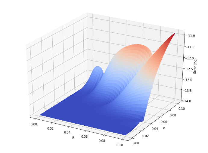
Compute $E$ from $M$

# We now investigate how accurate this map is around the nominal point
from mpl_toolkits.mplot3d import Axes3D
import matplotlib.pyplot as plt
from matplotlib import cm
from matplotlib.ticker import LinearLocator, FormatStrFormatter
import numpy as np

N = 50
M_grid = np.linspace(0,0.1,N)
e_grid = np.linspace(0,0.1,N)
# Make data.
X, Y = np.meshgrid(M_grid, e_grid)
Z = np.zeros([N,N])
for i in range(N):
    for j in range(N):
         res = E_map.evaluate({"dp0": X[i,j], "dp1": Y[i,j]}) + En
         Z[i,j] = np.log10(np.abs(X[i,j] - res + Y[i,j]*sin(res)) + 1e-14)

# Prepare the plot
fig = plt.figure(figsize=(12, 9))
ax = fig.gca(projection='3d')

# Plot the surface.
surf = ax.plot_surface(X, Y, Z, cmap=cm.coolwarm,
                       linewidth=0, antialiased=False)
ax.set_xlabel('E')
ax.set_ylabel('e')
ax.set_zlabel('Error (log)')
plt.show()